Two view reconstruction pipeline
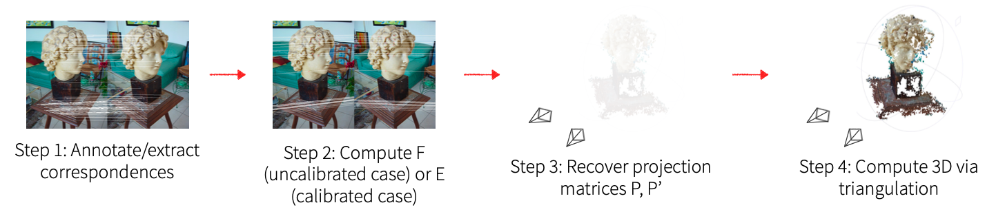
(Step 2) 8 points algorithm for computing fundamental matrix F and essential matrix E
8 points Algorithm
- Normalize all points to be centered at zero and a fixed average distance.
- For each point correspondence \(x, y\), set up linear equation \(y^{\top} F x = 0\) where \(F = \begin{bmatrix} f_1 & f_2 & f_3 \\ f_4 & f_5 & f_6 \\ f_7 & f_8 & 1 \\ \end{bmatrix}\)
- rewrite the equation as \(\begin{bmatrix}y_1x_1 & y_1x_2 & y_1x_3 & y_2x_1 & y_2x_2 & y_2x_3 & y_3x_1 & y_3x_2 & y_3x_3\end{bmatrix}\vec{f} = 0\)
- Stack all equations into matrix \(A\) of size \(N \times 9\).
- Solve \(Af = 0\) for \(f\) using SVD.
- Enforce rank-2 condition on \(f\) by taking only the first two singular values and then reshaping the last singular vector into \(3\times 3\) matrix \(\tilde{F}\).
- Apply unnormalization by applying the transformation matrices to \(\tilde{F}\): \(F = T_2^\top \tilde{F} T_1\)
- Compute \(E = K_2^{\top} F K_2\)
Results
| Chair | Teddy |
|---|---|
 |
 |
-
essential matrix E in chair scene \(\begin{bmatrix} 0.251 & -6.068 & -6.066 \\ 4.087 & 0.587 & -35.810 \\ 2.433 & 35.648 & 1. \\ \end{bmatrix}\)
-
essential matrix E in Teddy scene \(\begin{bmatrix} -5.369 & 20.941 & 77.113 \\ 1.930 & 13.211 & -180.207 \\ -31.719 & 185.536 & 1. \\ \end{bmatrix}\)
(Step 2) 7 points algorithm for computing the fundamental matrix F
7 points Algorithm
- Normalize all points to be centered at zero and a fixed average distance.
- For each point correspondence \(x, y\), set up linear equation \(y^{\top} F x = 0\) where \(F = \begin{bmatrix} f_1 & f_2 & f_3 \\ f_4 & f_5 & f_6 \\ f_7 & f_8 & 1 \\ \end{bmatrix}\)
- rewrite the equation as \(\begin{bmatrix}y_1x_1 & y_1x_2 & y_1x_3 & y_2x_1 & y_2x_2 & y_2x_3 & y_3x_1 & y_3x_2 & y_3x_3\end{bmatrix}\vec{f} = 0\)
- Stack all equations into matrix \(A\) of size \(7 \times 9\).
- Solve \(Af = 0\) for \(f\) using SVD.
- Take the last two singular vectors as \(F_1\) and \(F_2\), with the general solution being \(F = \lambda F_1 + (1-\lambda) F_2\).
- Find \(\lambda\) such that \(F\) satisfies \(\text{det}(F) = 0\):
- let \(f(\lambda) = \text{det}(\lambda F_1 + (1-\lambda) F_2)\) and \(g(\lambda) = a_3 \lambda^3 + a_2 \lambda^2 + a_1 \lambda + a_0\).
- Numerically calculate \(g\) in order to set up a system of four equations \(f(\lambda) = g(\lambda)\) and solve for \((a_3, a_2, a_1, a_0)\).
- Then solve \((\lambda) = a_3 \lambda^3 + a_2 \lambda^2 + a_1 \lambda + a_0 = 0\) for \(\lambda\).
- Take the real root and form solution \(\tilde{F} = \lambda F_1 + (1-\lambda) F_2\).
- Apply unnormalization by applying the transformation matrices to \(\tilde{F}\): \(F = T_2^\top \tilde{F} T_1\)
- Compute \(E = K_2^{\top} F K_2\)
Results
| Toybus | Toytrain |
|---|---|
 |
 |
(Step 2) RANSAC for 7 points and 8 points algorithms
RANSAC algorithm
- sample minimum required number of point correspondences (either 7 or 8)
- run the 7- or 8-points algorithm to find \(F\)
- check if the epipolar line \(l^\prime = Fx\) is close enough to the corresponding point \(x^\prime\) for each correspondence
- metric:
 l1, l2 = get_epipolar_lines(F, x1, x2)
 d1 = np.abs(l1.T @ to_projective(x1)) / np.linalg.norm(l1[:2])
 d2 = np.abs(l2.T @ to_projective(x2)) / np.linalg.norm(l2[:2])
 metric = d1 + d2
- metric:
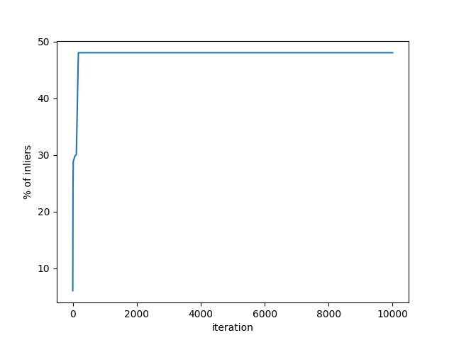
- count inliers: if epipolar line is close enough for more than 70% of the points, move to next step
- repeat previous step of counting inliers for the entire set of correspondences and keep the \(F\) if it fits more inliers than the previous best.
Results
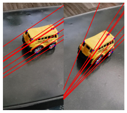
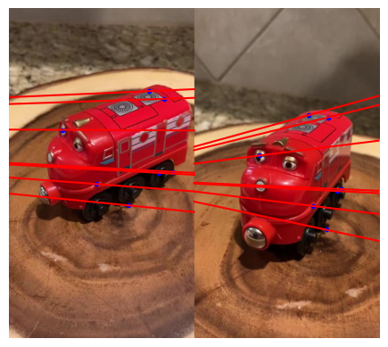
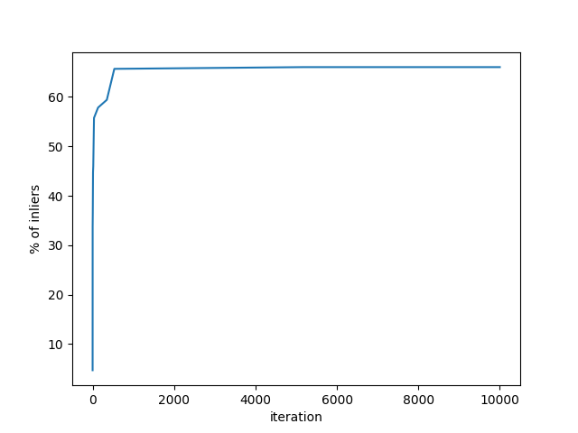
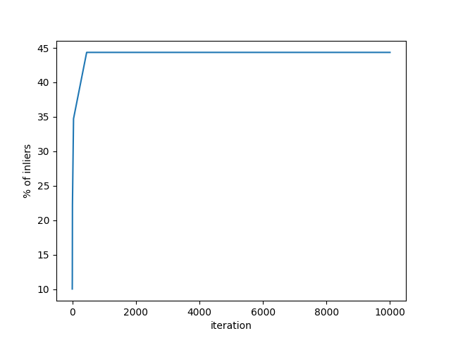
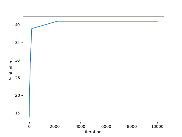
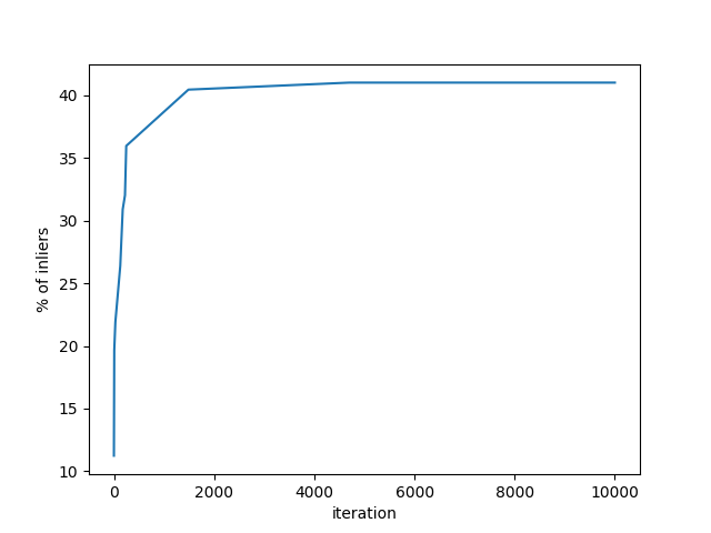
| Scene & algorithm | Epipolar lines | RANSAC progress (inlier count) |
|---|---|---|
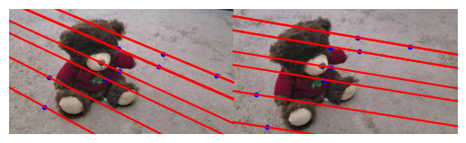
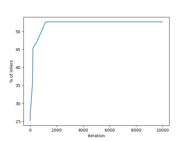
| Teddy (7-points) | 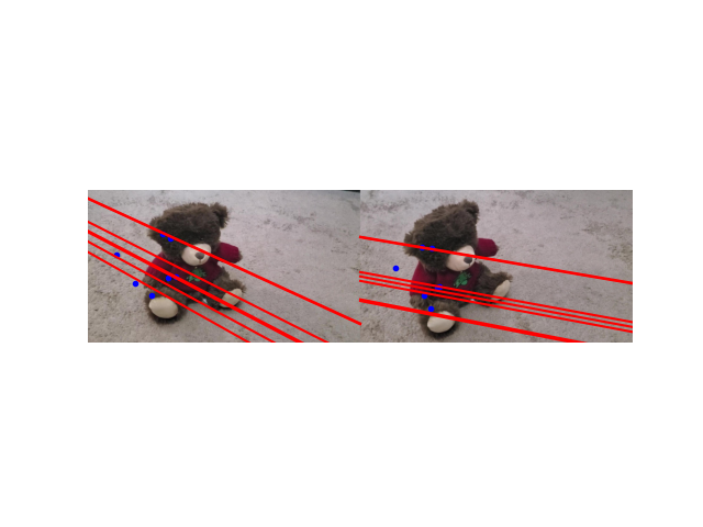 |
 |
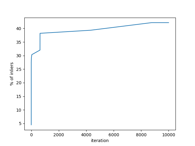
| Teddy (8-points) | 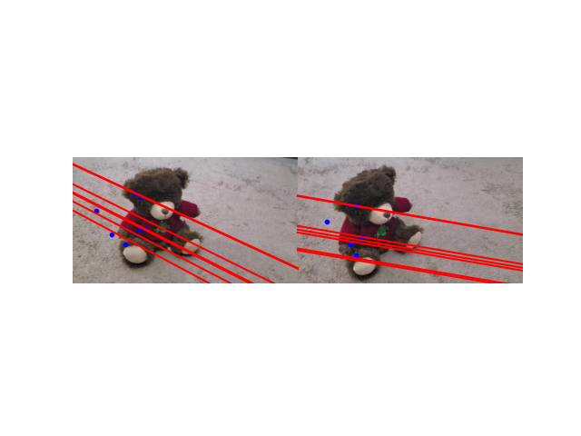 |
 |
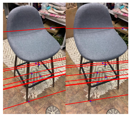
| Chair (7-points) |  |
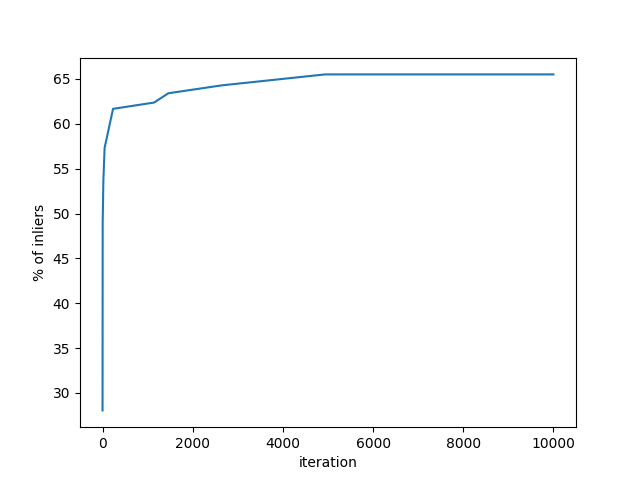 |
| Chair (8-points) | 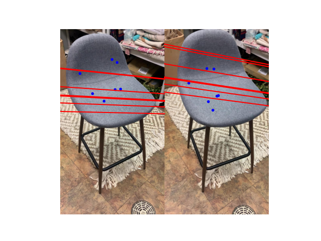 |
 |
| Toybus (7-points) |  |
 |
| Toybus (8-points) | 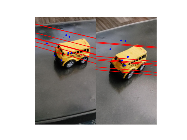 |
 |
| Toytrain (7-points) | 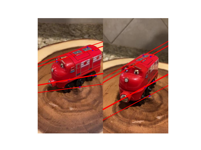 |
 |
| Toytrain (8-points) | 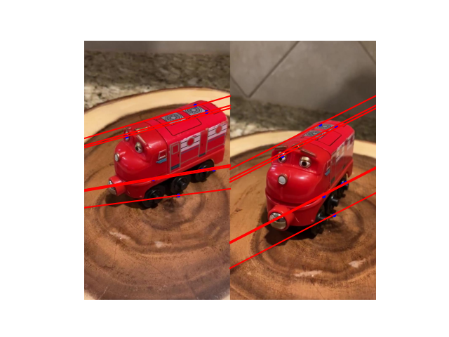 |
 |
(Step 4) Triangulation
Triangulation algorithm
- Normalize all points to be centered at zero and a fixed average distance.
- For each point correspondence \((x, y), (x^\prime, y^\prime)\) with camera projection matrices \(P, P^\prime\),
- write the equations as matrix \(A\) of size \(4 \times 4\). \(A = \begin{bmatrix} x \vec{p}^{3\top} - \vec{p}^{1\top} \\ y \vec{p}^{3\top} - \vec{p}^{2\top} \\ x^\prime \vec{p}^{\prime3\top} - \vec{p}^{\prime1\top} \\ y^\prime \vec{p}^{\prime3\top} - \vec{p}^{\prime2\top} \\ \end{bmatrix}\)
- Solve \(AX = 0\) for \(X\) using SVD.
- Take the last singular vector as \(X\).
Results
| Input 2D points | 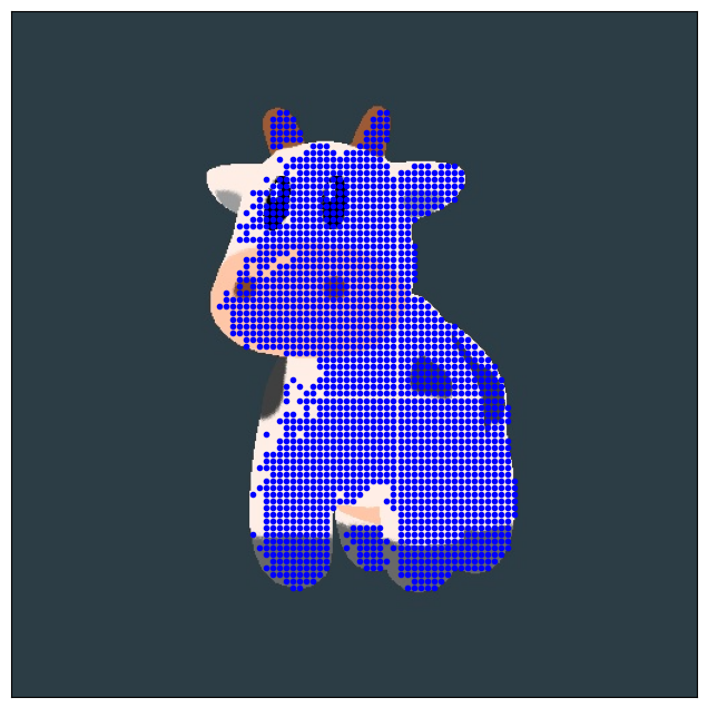 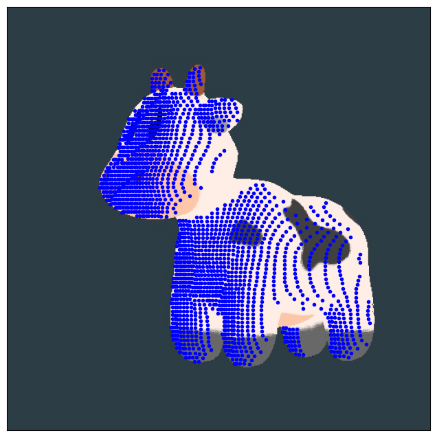 |
| Reconstructed 3D points |  |
(Step 2 and 5) COLMAP for Bundle Adjustment
Red points mark the estimated camera location at each frame, and black points mark the sparse reconstructed 3D points.
| input | output | |
|---|---|---|
| Burj Al Arab video source |
 |
 |
| Wat Muang Buddha video source |
 |
 |